Be2 PDFT Inversion - WuYang
[4]:
import numpy as np
import matplotlib.pyplot as plt
from CADMium import Pssolver, Psgrid, Partition, Inverter
[5]:
a = 4.522/2
#Nuclear charge for fragments A and B
Za, Zb = 4,4
#Set polarization 1-Unpolarized, 2-Polarized
pol = 1
#Fragment a electrons [alpha, beta]
Nmo_a = [[2]] #Number of molecular orbitals to calculate
N_a   = [[4]]
#Ensemble mix
nu_a = 1
#Fragment b electrons
Nmo_b = [[2]]
N_b   = [[4]]
#Ensemble mix
nu_b = 1

#Molecular elctron configuration
Nmo_m = [[4]]
N_m   = [[8]]


#Set up grid
NP = 7
NM = [6,6]
L = np.arccosh(15/a)
loc = np.array(range(-4,5)) #Stencil outline

grid = Psgrid(NP, NM, a, L, loc)
grid.initialize()

part = Partition(grid, Za, Zb, pol, Nmo_a, N_a, nu_a, Nmo_b, N_b, nu_b, { "kinetic_part_type" : "inversion",
                                                                          "ab_sym"            : True,
                                                                          "ens_spin_sym"      : False})
#Setup inverter object
mol_solver = Pssolver(grid, Nmo_m, N_m, {"tol_orbital" : 1e-9})
part.inverter = Inverter(grid, mol_solver, {"invert_type"    : "wuyang",
                                            "ab_sym"         : True,
                                            "ens_spin_sym"   : False,
                                            "tol_lin_solver" : 1e-3,
                                            "tol_invert"     : 1e-4,
                                            "res_factor"     : 0,
                                           })

part.optPartition.isolated = True
part.scf({"disp"  : False,
          "alpha" : [0.6],
          "e_tol" : 1e-7})

D0_frag_a = part.KSa.n.copy()
D0_frag_b = part.KSa.n.copy()

part.optPartition.isolated   = False
part.scf({"disp"       : True,
          "alpha"      : [0.3],
          "max_iter"   : 200,
          "e_tol"      : 1e-7,
          "continuing" : True,
          "iterative"  : False})

# #Store full densities under the presence of vp.
Dvp_frag_a = part.KSa.n.copy()
Dvp_frag_b = part.KSb.n.copy()
----> Begin SCF calculation for *Interacting* Fragments

                Total Energy (a.u.)                                Inversion

                __________________                ____________________________________

Iteration         A              B                  iters      optimality        res

___________________________________________________________________________________________

    1           -14.43315       -14.43315             5       +9.929e-02      +1.000e+00
    2           -14.43466       -14.43466             4       +2.091e-05      +1.556e-03
    3           -14.45966       -14.45966             4       +3.488e-04      +1.777e-03
    4           -14.43906       -14.43906             4       +7.463e-04      +1.847e-03
    5           -14.46721       -14.46721             3       +6.627e-03      +1.529e-03
    6           -14.44277       -14.44277             3       +2.213e-02      +1.032e-03
    7           -14.44361       -14.44361             3       +1.180e-02      +2.694e-04
    8           -14.43656       -14.43656             3       +1.373e-02      +6.894e-04
    9           -14.42236       -14.42236             3       +1.320e-02      +7.353e-04
   10           -14.41704       -14.41704             3       +7.746e-03      +6.876e-04
   11           -14.42367       -14.42367             3       +8.328e-03      +4.942e-04
   12           -14.43228       -14.43228             3       +9.280e-03      +2.459e-04
   13           -14.43920       -14.43920             3       +7.336e-03      +2.153e-04
   14           -14.44772       -14.44772             3       +1.101e-02      +3.033e-04
   15           -14.45136       -14.45136             3       +1.873e-02      +3.397e-04
   16           -14.44691       -14.44691             3       +3.135e-02      +2.411e-04
   17           -14.44188       -14.44188             3       +9.820e-03      +1.377e-04
   18           -14.43822       -14.43822             3       +6.350e-04      +8.514e-05
   19           -14.43457       -14.43457             2       +2.320e-02      +1.130e-04
   20           -14.43351       -14.43351             2       +2.596e-02      +1.247e-04
   21           -14.43566       -14.43566             2       +2.672e-02      +7.855e-05
   22           -14.43802       -14.43802             2       +2.550e-02      +6.005e-05
   23           -14.43954       -14.43954             2       +2.037e-02      +4.552e-05
   24           -14.44075       -14.44075             2       +1.329e-02      +5.106e-05
   25           -14.44087       -14.44087             2       +6.738e-03      +4.446e-05
   26           -14.43971       -14.43971             2       +3.407e-03      +3.569e-05
   27           -14.43860       -14.43860             2       +3.292e-03      +2.890e-05
   28           -14.43807       -14.43807             2       +3.827e-03      +3.107e-05
   29           -14.43781       -14.43781             2       +4.070e-03      +2.685e-05
   30           -14.43800       -14.43800             2       +3.290e-03      +1.770e-05
   31           -14.43865       -14.43865             2       +1.932e-03      +1.924e-05
   32           -14.43918       -14.43918             2       +7.566e-04      +1.837e-05
   33           -14.43936       -14.43936             2       +4.130e-04      +2.006e-05
   34           -14.43935       -14.43935             2       +4.281e-04      +1.529e-05
   35           -14.43916       -14.43916             2       +5.380e-04      +7.981e-06
   36           -14.43881       -14.43881             2       +5.464e-04      +1.010e-05
   37           -14.43855       -14.43855             2       +4.303e-04      +1.054e-05
   38           -14.43849       -14.43849             2       +2.412e-04      +1.128e-05
   39           -14.43853       -14.43853             2       +8.933e-05      +8.551e-06
   40           -14.43865       -14.43865             2       +5.332e-05      +4.024e-06
   41           -14.43882       -14.43882             2       +6.946e-05      +4.884e-06
   42           -14.43895       -14.43895             2       +9.087e-05      +4.876e-06
   43           -14.43897       -14.43897             2       +8.934e-05      +5.356e-06
   44           -14.43894       -14.43894             2       +6.197e-05      +4.212e-06
   45           -14.43888       -14.43888             2       +2.789e-05      +2.079e-06
   46           -14.43881       -14.43881             2       +9.303e-06      +2.150e-06
   47           -14.43875       -14.43875             2       +9.104e-06      +1.946e-06
   48           -14.43874       -14.43874             2       +1.284e-05      +2.176e-06
   49           -14.43876       -14.43876             2       +1.473e-05      +1.767e-06
   50           -14.43878       -14.43878             2       +1.233e-05      +9.149e-07
   51           -14.43881       -14.43881             2       +6.881e-06      +8.606e-07
   52           -14.43884       -14.43884             2       +2.423e-06      +7.434e-07
   53           -14.43884       -14.43884             2       +1.247e-06      +7.918e-07
   54           -14.43883       -14.43883             2       +1.642e-06      +6.373e-07
   55           -14.43882       -14.43882             2       +2.161e-06      +3.192e-07
   56           -14.43881       -14.43881             2       +2.170e-06      +3.181e-07
   57           -14.43880       -14.43880             2       +1.462e-06      +2.965e-07
   58           -14.43880       -14.43880             2       +6.386e-07      +2.871e-07
   59           -14.43881       -14.43881             2       +2.173e-07      +2.076e-07
   60           -14.43881       -14.43881             2       +2.015e-07      +9.987e-08
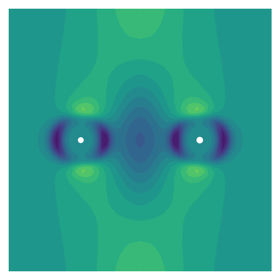
[7]:
full, x,y = grid.plotter(part.V.vp[:,0])
fig, ax = plt.subplots(dpi=300)

#vmin=-0.3, vmax=0.3

plot = ax.contourf(x,y,full, levels=20, cmap="viridis")
ax.scatter(4.522/2, 0, color='white', s=20)
ax.scatter(-4.522/2, 0, color='white', s=15)

ax.axis('off')


ax.set_aspect('equal')
ax.set_xlim([-5,5])
ax.set_ylim([-5,5])

# fig.colorbar(plot)
[7]:
(-5.0, 5.0)
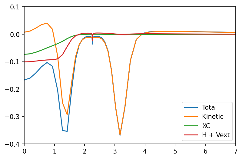
[8]:
x_axis, vp      = grid.axis_plot(part.V.vp[:,0])
x_axis, vp_kin  = grid.axis_plot(part.V.vp_kin[:,0])
x_axis, vp_xc   = grid.axis_plot(part.V.vp_x[:,0] + part.V.vp_c[:,0] )
x_axis, vp_hext = grid.axis_plot( part.V.vp_h[:,0] + part.V.vp_pot[:,0])

fig, ax = plt.subplots(dpi=150)

ax.plot(x_axis, vp, label='Total')
ax.plot(x_axis, vp_kin, label='Kinetic')
ax.plot(x_axis, vp_xc, label='XC')
ax.plot(x_axis, vp_hext, label="H + Vext")

ax.set_xlim(0,7)
ax.set_ylim(-0.4, 0.1)

ax.legend()
[8]:
<matplotlib.legend.Legend at 0x7f73e3381520>
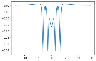
[11]:
x = x_axis
plt.plot(x, vp)
[11]:
[<matplotlib.lines.Line2D at 0x7f73e0da2e50>]
[19]:
# np.save('y.npy',  x)
# np.save('d1.npy', d1)
# np.save('d2.npy', d2)
np.save('vp.npy',vp)
[15]:
x, d1      = grid.axis_plot(part.KSa.n[:,0])
x, d2      = grid.axis_plot(part.KSb.n[:,0])
[16]:
plt.plot(x, d1)
plt.plot(x, d2)
[16]:
[<matplotlib.lines.Line2D at 0x7f73e0d4e250>]
