Li2 PDFT Inversion - Orbital Invert
[1]:
import numpy as np
import matplotlib.pyplot as plt
from CADMium import Kohnsham, Pssolver, Psgrid, Partition, Inverter
Perform PDFT Calculation. Currently the method used is “OrbitalInvert”. But original code may have used “WuYang”. Code should run as it is but for idential calculations increase to grid size to: [7,12,12]
[2]:
a = 5.122/2
#Nuclear charge for fragments A and B
Za, Zb = 3,3
#Set polarization 1-Unpolarized, 2-Polarized
pol = 2
#Fragment a electrons [alpha, beta]
Nmo_a = [[2,1]] #Number of molecular orbitals to calculate
N_a   = [[2,1]]
#Ensemble mix
nu_a = 1
#Fragment b electrons
Nmo_b = [[2,1]]
N_b   = [[2,1]]
#Ensemble mix
nu_b = 1

#Molecular elctron configuration
Nmo_m = [[3,3]]
N_m   = [[3,3]]

#Grid Options
NP = 7 #Number of points per block
NM =  [6,6] #Number of blocks [angular, radial]
L = np.arccosh(15./a) #Maximum radial coordinate value
loc = np.array(range(-4,5)) #Non inclusive on upper bound
grid = Psgrid(NP, NM, a, L, loc)
grid.initialize()


#Initialize required objects. And make calculation in isolated fragments for initial guess.

part = Partition(grid, Za, Zb, pol, Nmo_a, N_a, nu_a, Nmo_b, N_b, nu_b, { "kinetic_part_type" : 'inversion',
                                                                          "vp_calc_type"      : "component",
                                                                          "ab_sym"            : True,
                                                                          "ens_spin_sym"      : True,})

#Setup inverter object
mol_solver = Pssolver(grid, Nmo_m, N_m)
part.inverter = Inverter(grid, mol_solver, {"invert_type"     : "orbitalinvert",
                                            "tol_invert"      : 1e-10,
                                            "max_iter_invert" : 100,
                                            "disp"            : False,
                                            "ab_sym"          : True,
                                            "ens_spin_sym"    : True,})

part.optPartition.isolated = True
part.scf({"disp"  : False,
          "alpha" : [0.6],
          "e_tol" : 1e-12})

D0_frag_a = part.KSa.n.copy()
D0_frag_b = part.KSa.n.copy()


#Turn off iterative linear solver for each solver
part.KSa.solver[0][0].optSolver.iter_lin_solver = False
part.KSa.solver[0][1].optSolver.iter_lin_solver = False


part.optPartition.isolated   = False

part.scf({"disp"       : True,
          "alpha"      : [0.6],
          "max_iter"   : 200,
          "e_tol"      : 1e-9,
          "continuing" : True})

#Store full densities under the presence of vp.
Dvp_frag_a = part.KSa.n.copy()
Dvp_frag_b = part.KSb.n.copy()
----> Begin SCF calculation for *Interacting* Fragments

                Total Energy (a.u.)                                Inversion

                __________________                ____________________________________

Iteration         A              B                  iters      optimality        res

___________________________________________________________________________________________

    1            -7.32464        -7.32464             9       +4.669e-11      +1.000e+00
    2            -7.32866        -7.32866            10       +2.640e-11      +4.569e-02
    3            -7.34060        -7.34060             8       +2.320e-11      +2.900e-02
    4            -7.34060        -7.34060             9       +6.667e-15      +2.343e-02
    5            -7.33583        -7.33583             8       +5.507e-14      +9.256e-03
    6            -7.33822        -7.33822             6       +5.684e-11      +6.618e-03
    7            -7.33610        -7.33610             6       +2.891e-12      +7.186e-03
    8            -7.33881        -7.33881             6       +5.221e-13      +4.741e-03
    9            -7.33881        -7.33881             6       +4.692e-14      +4.233e-03
   10            -7.33747        -7.33747             6       +3.988e-14      +1.798e-03
   11            -7.33727        -7.33727             5       +6.818e-15      +2.017e-03
   12            -7.33780        -7.33780             5       +4.633e-15      +2.049e-04
   13            -7.33806        -7.33806             4       +1.979e-14      +9.114e-04
   14            -7.33787        -7.33787             4       +1.868e-11      +2.684e-04
   15            -7.33769        -7.33769             4       +7.529e-13      +2.949e-04
   16            -7.33770        -7.33770             4       +1.610e-13      +1.668e-04
   17            -7.33779        -7.33779             4       +2.142e-14      +7.718e-05
   18            -7.33782        -7.33782             3       +3.512e-15      +7.973e-05
   19            -7.33780        -7.33780             3       +7.010e-15      +1.557e-05
   20            -7.33778        -7.33778             3       +6.368e-15      +3.423e-05
   21            -7.33778        -7.33778             3       +5.012e-15      +6.247e-06
   22            -7.33778        -7.33778             2       +6.697e-11      +1.409e-05
   23            -7.33778        -7.33778             3       +5.048e-15      +4.038e-06
   24            -7.33778        -7.33778             2       +1.795e-11      +5.011e-06
   25            -7.33779        -7.33779             2       +1.820e-11      +2.902e-06
   26            -7.33779        -7.33779             2       +4.423e-12      +1.351e-06
   27            -7.33779        -7.33779             2       +1.832e-12      +1.447e-06
   28            -7.33778        -7.33778             2       +1.640e-12      +2.644e-07
   29            -7.33778        -7.33778             2       +4.237e-14      +6.179e-07
   30            -7.33778        -7.33778             2       +1.793e-13      +1.044e-07
   31            -7.33778        -7.33778             2       +2.103e-14      +2.435e-07
   32            -7.33778        -7.33778             2       +3.179e-14      +8.058e-08
   33            -7.33778        -7.33778             2       +3.674e-15      +8.225e-08
   34            -7.33778        -7.33778             2       +6.347e-15      +5.243e-08
   35            -7.33778        -7.33778             2       +4.465e-15      +2.293e-08
   36            -7.33778        -7.33778             2       +4.829e-15      +2.604e-08
   37            -7.33778        -7.33778             2       +3.640e-15      +4.308e-09
   38            -7.33778        -7.33778             2       +5.013e-15      +1.112e-08
   39            -7.33778        -7.33778             2       +4.546e-15      +1.868e-09
   40            -7.33778        -7.33778             1       +5.572e-11      +3.127e-09
   41            -7.33778        -7.33778             1       +7.961e-11      +3.317e-09
   42            -7.33778        -7.33778             2       +5.179e-15      +1.781e-09
   43            -7.33778        -7.33778             1       +6.557e-11      +3.011e-09
   44            -7.33778        -7.33778             2       +6.550e-15      +1.382e-09
   45            -7.33778        -7.33778             1       +3.592e-11      +2.160e-09
   46            -7.33778        -7.33778             2       +4.416e-15      +8.979e-10
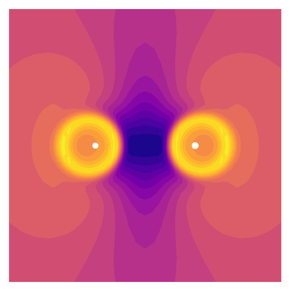
Generate Figure 9. Parititon Potential.
[3]:
full, x,y = grid.plotter(part.V.vp[:,0])
fig, ax = plt.subplots(dpi=300)

plot = ax.contourf(x,y,full, levels=22, cmap="plasma")

ax.set_aspect('equal')
ax.set_xlim([-7,7])
ax.set_ylim([-7,7])

ax.scatter(5.122/2, 0, color='white', s=20)
ax.scatter(-5.122/2, 0, color='white', s=15)

ax.axis('off')

# fig.colorbar(plot)
# plt.show()
[3]:
(-7.0, 7.0, -7.0, 7.0)
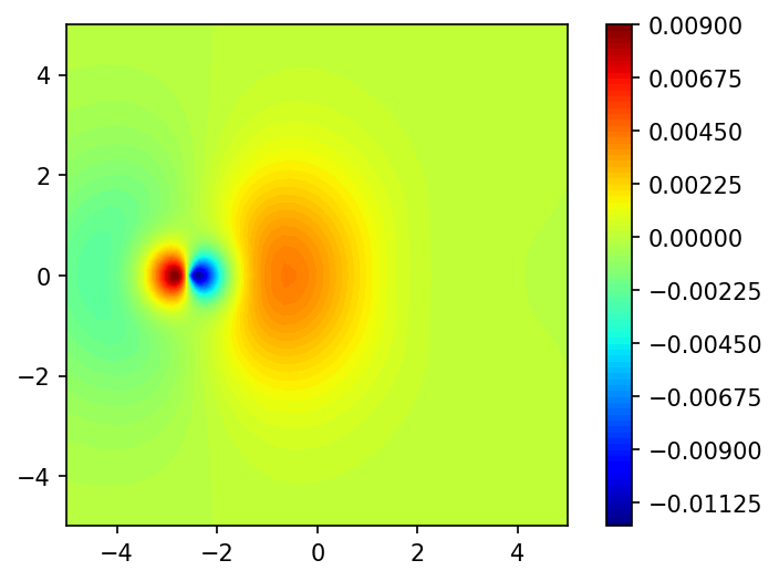
Generate Figure 9. Difference between Fragment Density and Isolated Atomic Density.
[4]:
D_grid, x, y = grid.plotter(D0_frag_a[:,0])
D_vp_grid, _, _ = grid.plotter(Dvp_frag_a[:,0])

fig, ax = plt.subplots(dpi=150)
plot = plt.contourf(x,y, D_vp_grid - D_grid, levels=100, cmap="jet")

ax.set_aspect('equal')
ax.set_xlim([-5,5])
ax.set_ylim([-5,5])

fig.colorbar(plot)
# plt.show()
[4]:
<matplotlib.colorbar.Colorbar at 0x7fd6d81e1b80>
Generate Figure 11. Components of the Partition Potential
[13]:
x_axis, vp      = grid.axis_plot(part.V.vp[:,0])
x_axis, vp_kin  = grid.axis_plot(part.V.vp_kin[:,0])
x_axis, vp_xc   = grid.axis_plot(part.V.vp_x[:,0] + part.V.vp_c[:,0] )
x_axis, vp_hext = grid.axis_plot( part.V.vp_h[:,0] + part.V.vp_pot[:,0])

fig, ax = plt.subplots(dpi=150)

ax.set_title("Li$_2$")
ax.axvline(x=a, color="gray", ls=':', alpha=0.5)

ax.plot(x_axis, vp,  label='$v_p(r)$', lw=4, color="#FD9903")
# ax.plot(x_axis, vp_kin, label='Kinetic')
# ax.plot(x_axis, vp_xc, label='XC')
# ax.plot(x_axis, vp_hext, label="H + Vext")

ax.set_xlim(0,7)
ax.set_ylim(-0.12, 0.12)

ax.legend()

plt.plot
[13]:
<function matplotlib.pyplot.plot(*args, scalex=True, scaley=True, data=None, **kwargs)>
Generate Table 9. Energies and Components of Ep, in atomic Units
[6]:
values = {}
for i in part.E.__dict__:
    if i.startswith("__") is False:
        values.update({i : getattr(part.E, i)})
values
[6]:
{'Ea': -7.337784849443342,
 'Eb': -7.337784849443342,
 'Ef': -14.675569698886685,
 'Tsf': 14.51597760325188,
 'Eksf': array([[-3.87274135, -3.62105118]]),
 'Enucf': -33.88821469087027,
 'Exf': -3.0418434859179895,
 'Ecf': -0.30099393918618395,
 'Ehf': 8.03950481383588,
 'Vhxcf': 11.684634289090774,
 'Ep': -1.8069182239952444,
 'Ep_pot': -3.678211853854383,
 'Ep_kin': 0.004784336086627761,
 'Ep_hxc': 1.8665092937725107,
 'Et': -16.48248792288193,
 'Vnn': 1.757126122608356,
 'E': -14.725361800273573,
 'evals_a': array([-1.8178079 , -0.11856278, -1.81052559]),
 'evals_b': array([-1.8178079 , -0.11856278, -1.81052559]),
 'Ep_h': 1.886610621676736,
 'Ep_x': 0.007092235124383617,
 'Ep_c': -0.02719356302860887}
[7]:
%matplotlib widget

fig, ax = plt.subplots(subplot_kw={"projection": "3d"}, dpi=300)
surf = ax.plot_surface(x, y, full, cmap="plasma", alpha=1.0,
                       linewidth=20, antialiased=True)

ax.grid(False)
ax.set_axis_off()
ax.dist = 6
ax.set_facecolor("white")

fig.show()